
Magnetic fields are completely invisible to the naked eye—which makes understanding how they work a real challenge.
That’s where visual science comes in.
If you are looking for clear, accurate pictures of a magnetic field, you’ve come to the right place. In this guide, we’ve gathered the most striking visual representations of magnetic forces in action—from classic iron filing patterns to cutting-edge 3D simulations.
Let’s dive right in!
How Do We Capture Pictures of a Magnetic Field?
Magnetic fields dictate how modern electronics, motors, and magnetic assemblies perform, yet their force lines remain hidden from our sight. Capturing pictures of a magnetic field requires transforming invisible flux lines and field density into visible, measurable formats.
+————————————————————-+
| Magnetic Field Visualization |
+——————————+——————————+
| Physical Flux Visualizers | Digital Sensor Scans |
| (Viewing film, ferrofluid) | (Hall arrays, FEA models) |
| * Shows layout & poles | * Measures flux density |
+——————————+——————————+
Why Magnetic Fields Are Invisible to the Naked Eye
Magnetic fields represent vector force distributions generated by moving electric charges and aligned electron spins in materials like Neodymium (NdFeB), Ferrite, or SmCo.
-
- No Optical Interaction: Magnetic flux lines do not emit, absorb, or scatter photons within the visible light spectrum.
- Continuous Vector Fields: A magnetic field is an invisible spatial gradient of flux density rather than a solid boundary.
- Medium Dependency: To capture a photo, we must introduce a responsive medium—such as micro-encapsulated nickel flakes, ferrofluids, or calibrated Hall effect sensor arrays—that physically or digitally reacts to the field vectors.
Direct Physical Visualizers vs. Digital Sensor Mapping
We generally split magnetic field imagery into two primary engineering approaches:
-
- Direct Physical Visualizers:
- Tools like magnetic viewing film use liquid-suspended nickel/iron flakes that physically pivot to expose magnetic pole boundaries, transitions, and multi-pole patterns immediately.
- Simple, quick for production checks, and ideal for spotting surface cracks or irregular magnetization.
- Digital Sensor Mapping:
- Uses 2D or 3D Hall sensor arrays and magnetic field scanning cameras.
- Measures precise quantitative values (Gauss or Tesla) and generates false-color intensity maps showing exact flux gradient distributions.
Real Photos, Field Line Simulations, and Data Models
Understanding what a magnetic field image represents helps in choosing the right tool for design validation and quality control:
| Imaging Method | How It Works | Best Used For | Output Type |
|---|---|---|---|
| Physical Visualizer Film | Flakes align mechanically along flux lines | Instant pole identification, crack detection | Real photographic image |
| Digital Sensor Mapping | Multi-axis Hall probes scan surface field points | Quantitative flux density (Br) verification | 2D/3D color-coded data map |
| FEA Simulation Models | Finite Element Analysis calculates theoretical lines | Magnetic circuit design, Halbach array planning | Computer-generated vector model |
Classic Methods to Visualize and Photograph Magnetic Fields
Capturing clear pictures of a magnetic field doesn’t always require lab-grade digital scanners. We often rely on practical physical tools to make invisible flux lines tangible, photo-ready, and easy to inspect.
Iron Filings on Paper: Capturing Bar and Horseshoe Magnet Lines
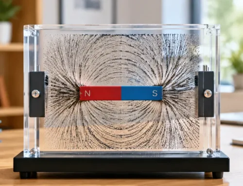
The classic iron filing method remains one of the simplest ways to map out field geometry.
Kako deluje: Sprinkling fine iron particles onto a sheet of paper or glass suspended over a magnet causes each particle to act like a tiny dipole.
Visual result: The filings align along flux vectors, producing a crisp 2D bar magnet field picture or the dense, looping curves of a classic horseshoe magnet field pattern.
Photography tip: Use side lighting (raking light) against a white backdrop to cast small shadows under each grain, adding depth and contrast to your photo.
Ferrofluid Photography: Creating 3D Liquid Magnetic Spikes
For striking 3D imagery, liquid ferrofluid photography brings magnetic flux lines into physical relief.
The mechanism: Ferrofluid contains nanoscale iron oxide particles suspended in a carrier fluid with a surfactant. When exposed to a magnetic field, the balance between surface tension and magnetic pull creates dynamic spikes along the field lines.
Visual result: Volumetric, needle-like formations that follow the local field strength, making high-intensity flux peaks immediately visible to the camera.
Magnetic Viewing Film: Exposing Hidden Pole Patterns
When we inspect modern permanent magnets—such as multi-pole rings or assemblies found in a magnetic door latch and types of magnets used in commercial hardware—standard iron filings are too messy.
Kako deluje: Magnetic viewing film uses micro-encapsulated nickel or iron flakes suspended in liquid between flexible plastic sheets.
Visual result: The film turns dark green along pole transitions and light green over magnetic poles, instantly revealing multi-pole spacing, cracks, and field orientation.
Miniature Compass Arrays: Plotting Directional Field Vectors
While filings show the lines, they don’t show the vector direction.
Kako deluje: Placing a grid of micro-magnetic compasses around a test magnet forces each needle to point from North to South along local lines of force.
Visual result: A clean, vector-mapped graphic of magnetic polarity across an entire plane, perfect for step-by-step educational captures and quick polarity verification.
Advanced and Scientific Magnetic Field Imagery
Capturing true pictures of a magnetic field on a grand scale—or down at the atomic level—requires specialized scientific instruments. When physical films or filings cannot reach, advanced imaging sensors and electron optics translate invisible magnetic forces into highly detailed visual records.
Earth’s Magnetosphere: How Satellites Map Planetary Fields
Planetary fields cannot be photographed with standard optical sensors. Instead, space agencies use satellite magnetometer arrays and particle detectors to generate comprehensive Earth magnetosphere images:
-
- In-situ sensor networks: Satellites record local field vector data, direction, and magnetic flux density lines across orbital paths.
- Data-driven visual rendering: Supercomputers convert real-time field data into false-color 3D models showing the compressed dayside shield and the elongated magnetotail reacting to solar winds.
Solar Magnetic Field Pictures: Capturing Coronal Loops
The Sun provides some of the most dynamic magnetic imagery in the solar system. Extreme ultraviolet (EUV) telescopes capture massive plasma streams trapped along solar magnetic loops:
-
- Plasma tracing: Glowing, superheated plasma flows directly along twisted field lines, revealing giant arching structures above active sunspot regions.
- Magnetograms: Spacecraft map polarized light shifts (Zeeman effect) to render high-contrast black-and-white images, where white patches mark outgoing positive flux and black patches mark incoming negative flux.
Electron Holography and Lorentz Microscopy: Nanoscale Domains
To view nanoscale magnetic structures inside high-performance permanent magnets, advanced laboratories rely on transmission electron microscopy:
-
- Lorentz microscopy magnetic domain imaging: Transmitted electron beams bend slightly when passing through local magnetic fields, creating bright and dark boundary lines at domain walls.
- Electron holography: Measures the phase shift of electron waves passing through magnetic materials, producing detailed phase-contour maps that show exact magnetic flux paths inside thin films and sintered magnet grains—much like microscopic versions of classic bar magnet magnetic field paths.
MRI Magnetic Field Mapping in Medical Diagnostic Imaging
Magnetic Resonance Imaging (MRI) relies on uniform, stable magnetic fields generated by superconducting coils. Field mapping ensures image clarity and patient safety:
-
- Phase-shift field maps: Diagnostic systems generate 2D and 3D field-homogeneity maps by analyzing phase shifts of hydrogen protons in the scanner bore.
- Gradient verification: These false-color intensity maps highlight micro-distortions, allowing engineers to correct non-linearities before scanning delicate biological tissues.
DIY Guide: Taking Pictures of a Magnetic Field at Home
Capturing clear pictures of a magnetic field does not require an advanced research laboratory. With a few affordable materials and the right camera setup, we can photograph stunning, high-contrast magnetic flux lines right from a workbench or desk.
Essential Gear: Strong Neodymium Magnets, Iron Powder, Glass, and Lighting
To get clean, defined results, assemble these basic components:
-
- Strong Neodymium Magnets: High-grade NdFeB blocks, discs, or rings generate the field strength needed to align particles crisply. These powerful fields are the same principles utilized in high-precision microrobot and neodymium magnets systems.
- Fine Iron Powder or Filings: Uniform, fine-mesh iron powder creates continuous, clean lines rather than clunky clusters.
- Clear Glass or Acrylic Sheet: A rigid, transparent barrier placed over the magnet keeps the iron clean and allows effortless resetting between shots.
- Directional LED Lighting: A controllable light source helps bring out fine particle textures and depth.
Lighting and Contrast Techniques to Highlight Micro-Details
Standard overhead room lighting washes out the micro-textures of magnetic field lines. To capture deep, dramatic images:
-
- Use Low-Angle Raking Light: Position your LED light source at a shallow side angle (15° to 30° relative to the glass). This casts microscopic shadows behind each aligned iron particle, giving the field lines a tangible 3D appearance.
- Control the Background: Place a sheet of matte white acrylic under the glass for dark iron filings, or use a matte black surface when photographing reflective metallic powders or ferrofluid.
- Diffuse Hotspots: Place a piece of tracing paper or a light diffuser in front of your LED to eliminate harsh reflections off the glass surface.
Step-by-Step Setup to Safely Photograph Ferrofluid in Action
Ferrofluid provides spectacular liquid spikes along magnetic lines, but it stains surfaces quickly. Follow this controlled setup:
-
- Contain the Fluid: Place a shallow, clear glass petri dish or shallow watch glass on your stand.
- Add the Carrier Medium: Pour a thin layer of distilled water or light mineral oil into the dish to prevent the ferrofluid from sticking to the bottom glass.
- Dispense Carefully: Use a pipette to deposit 2 to 3 drops of ferrofluid into the center of the liquid.
- Introduce the Magnetic Field: Slowly raise a neodymium magnet underneath the bottom of the dish. Watch the smooth liquid instantly form sharp geometric spikes following the field vectors.
- Adjust the Gap: Fine-tune the distance between the magnet and the glass to balance spike height and prevent splashing onto the magnet.
Smartphone Camera Macro Settings for Sharp Magnetic Field Lines
Modern smartphone cameras can capture incredible close-up detail if you dial in the right manual controls:
-
- Switch to Macro or Pro Mode: Lock the focus manually directly on the apex of the field lines or ferrofluid spikes to prevent the autofocus from hunting.
- Drop the ISO: Set the ISO manually to the lowest setting (ISO 50 or 100) to eliminate digital grain and preserve edge sharpness.
- Stabilize the Shot: Mount the phone on a compact tripod and use a 2-second shutter delay. This completely removes hand-shake blur during close-up macro shots.
- Adjust Exposure Bias: Slightly lower the exposure compensation (-0.3 to -0.7 EV) to keep the brightest highlights on metallic particles from blowing out.
How to Read and Interpret Pictures of a Magnetic Field
When we look at pictures of a magnetic field, we are viewing a visual map of invisible force paths. Knowing how to read these patterns helps us quickly evaluate pole alignment, field intensity, and potential flux leakage.
Understanding Line Density and Field Strength (Flux Density)
Visual representations use spatial density or color saturation to convey magnetic flux density:
-
- High line density: Where lines are tightly packed together—typically right at the magnet edges and pole faces—the magnetic force is at its strongest.
- Low line density: As lines diverge and spread outward into surrounding space, the field rapidly weakens.
- Color heatmaps: In digital sensor imaging, warm colors (reds and yellows) denote peak flux density, while cooler tones (blues and greens) represent dropping field values.
Identifying Attraction vs. Repulsion Patterns Between Poles
Analyzing interaction zones reveals pole orientations immediately:
-
- Attraction (Opposite Poles): Continuous field lines bridge directly across the gap from North to South, pulling the visual markers into smooth, connecting arches.
- Repulsion (Like Poles): Lines bend sharply away from each other without crossing, leaving a distinct blank or zero-field neutral zone right in the center between the two repelling faces.
Spotting Uniform vs. Non-Uniform Magnetic Field Behaviors
Field geometry reveals how evenly the magnetic force performs across a target area:
-
- Uniform magnetic fields: Characterized by straight, parallel, and evenly spaced lines. We see this consistent behavior inside the core of solenoids or within narrow gaps between broad, flat pole pieces.
- Non-uniform magnetic fields: Characterized by curved, diverging, or asymmetrical line distribution. Standard point poles or specialized multi-pole setups exhibit steep field gradients, just like when we analyze the concentrated strength of the Halbach array magnet field on one side while the opposite side cancels out.
Frequently Asked Questions About Magnetic Field Pictures
Can a normal digital camera see magnetic fields directly?
No, standard digital cameras cannot capture magnetic fields directly. Digital camera sensors (CMOS and CCD) only detect photons across visible, infrared, and ultraviolet light spectrums. Because magnetic fields do not emit or reflect visible light on their own, we must use an intermediary medium to make them visible. To get clear pictures of a magnetic field, we rely on physical visualizers like iron filings, specialized films, or multi-axis electronic sensors that convert field intensity into visual data.
What is the green paper used to picture magnetic fields?
That green sheet is magnetic viewing film (also known as flux detector film). It consists of micro-encapsulated nickel or iron flakes suspended in a liquid layer.
-
- Kako deluje: When we place the film directly over a magnet, the microscopic flakes rotate and align along the magnetic flux lines.
- What you see: Regions where flux lines are perpendicular to the surface appear dark, while areas with horizontal flux lines appear light green.
- Pogoste uporabe: It gives an instant visual layout of pole transitions, crack defects, and multi-pole patterns when inspecting components or learning what is the use of magnetic bar assemblies.
Why does ferrofluid form spikes in magnetic field photos?
The striking spikes in ferrofluid photography happen because of a physical phenomenon called normal-field instability (or Rosensweig instability).
-
- Magnetic pull: Nanoscale magnetic particles inside the carrier fluid get pulled upward along the lines of maximum magnetic field strength.
- Surface tension balance: Surface tension and gravity try to keep the liquid flat.
- The result: The liquid finds an energetic equilibrium by forming regular geometric cones that follow the magnetic vector paths.
How do scientists capture color images of invisible magnetic fields?
Scientific color imagery of magnetic fields relies on digital sensor mapping rather than standard photography:
-
- Hall sensor arrays: 2D and 3D magnetic scanning cameras sweep across the magnetic surface, measuring exact flux density ($B_r$) and direction at thousands of grid points.
- False-color mapping: Software converts the numerical data into a high-resolution color map.
- Color grading: High-flux North poles are typically assigned warm colors (like red or orange), South poles appear in cool tones (like deep blue), and neutral transition zones show up in green or yellow.



 Slovenian
  English
  German
  Vietnamese
  Spanish (Mexico)
  Russian
  Turkish
  Polish
  Hindi
Hindi  Thai
Thai  Malay
Malay  Korean
  Japanese
  French
  Czech
Czech  Danish
  Dutch
Dutch  Finnish
  Italian
  Portuguese (Brazil)
  Portuguese (Portugal)
  Ukrainian
  Hebrew
  Scottish Gaelic
  Hungarian
  Tagalog
  Spanish (Spain)
  Serbian
  Indonesian
  Slovak
  Dutch (Belgium)
  Persian
  Arabic
  Romanian
  Estonian
  Greek
Greek  Bulgarian



Pusti komentar